Large 3 “Travel through Another Dimension”
A Basic Slicer for 3D Printing
Part 1
Task 1
Overview
The script can be downloaded here.

Single Layer Test
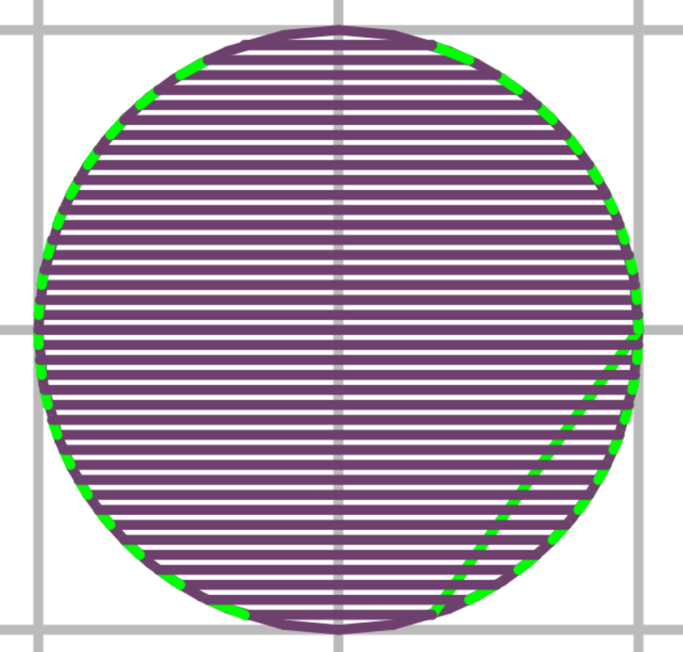
The image below shows a single slice from the output of my slicer. Purple lines are extrusion and green lines are travels.
Multi-Layer Test
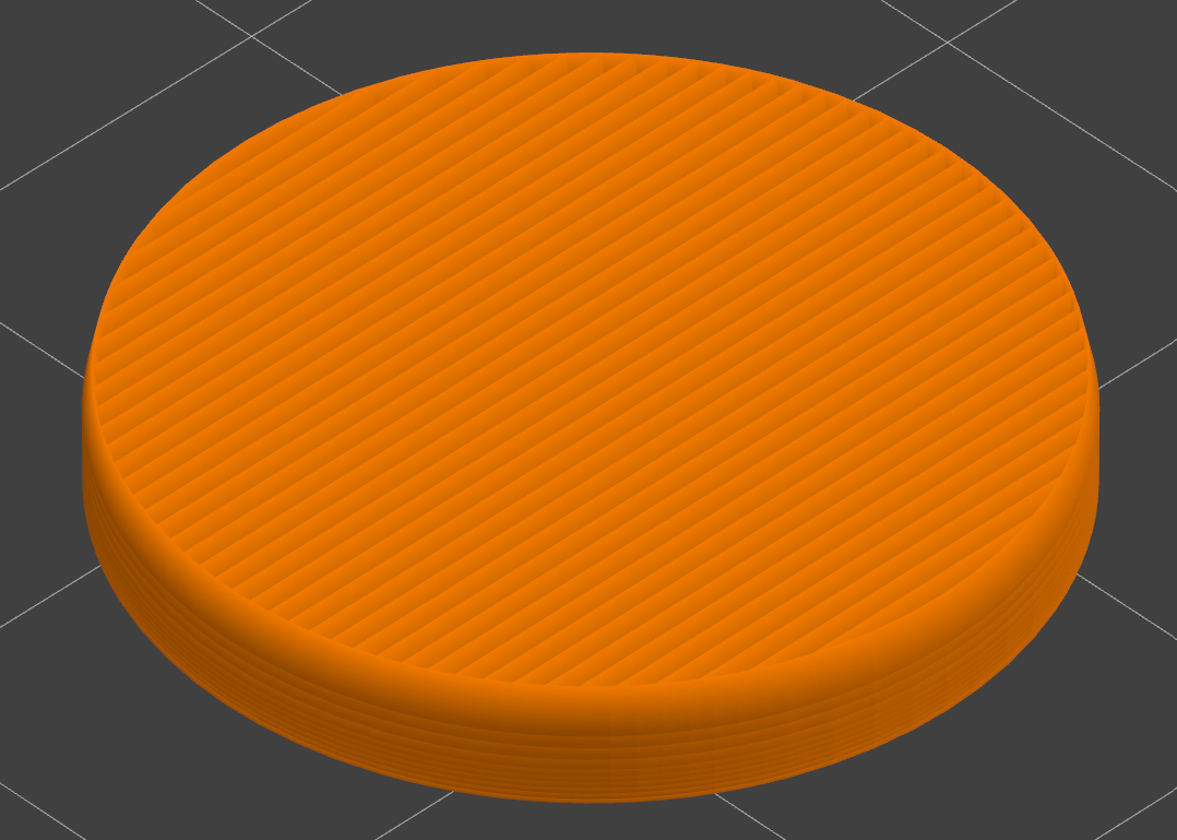
The image below shows multiple slices from the output of my slicer. This image is from Prusa Slicer visualization (I imported my gcode) and properly renders the extrusion width being calculated correctly.
Task 2
The gcode_move() function
The generate_gcode() function
Converting perimeters and infill to polylines
This function combines the perimeters and infill lines into polylines for gcode generation.
Line Infill Pattern Generation
To generate the line infill pattern, I started with a Python block. This block takes several parameters: the minimum and maximum 2D coordinates of a bounding box around the geometry, the bead width, and the infill density percentage (see extra credit). My Python function uses this information to generate a line pattern within the bounding box. The Python function returns the unclipped lines. I then use the sliced perimeters and a “Trim With Region” block to cut the lines to fit the geometry. The infill lines will eventually be paired with the perimeters before G-code generation. The image below shows the Grasshopper program, and the code shows the Python code used. My function also allows for lines to be generated horizontal or vertical.

Task 3
Single Layer Test
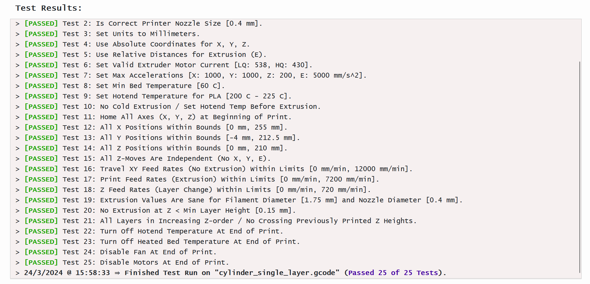
The image below shows the test result from my slicer. All tests were passed.
The full gcode can be accessed here.
Multi-Layer Test
The image below shows the test result from my slicer. All tests were passed.
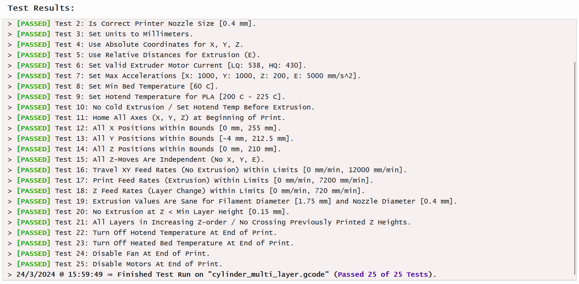
The full gcode can be accessed here.
Part 2
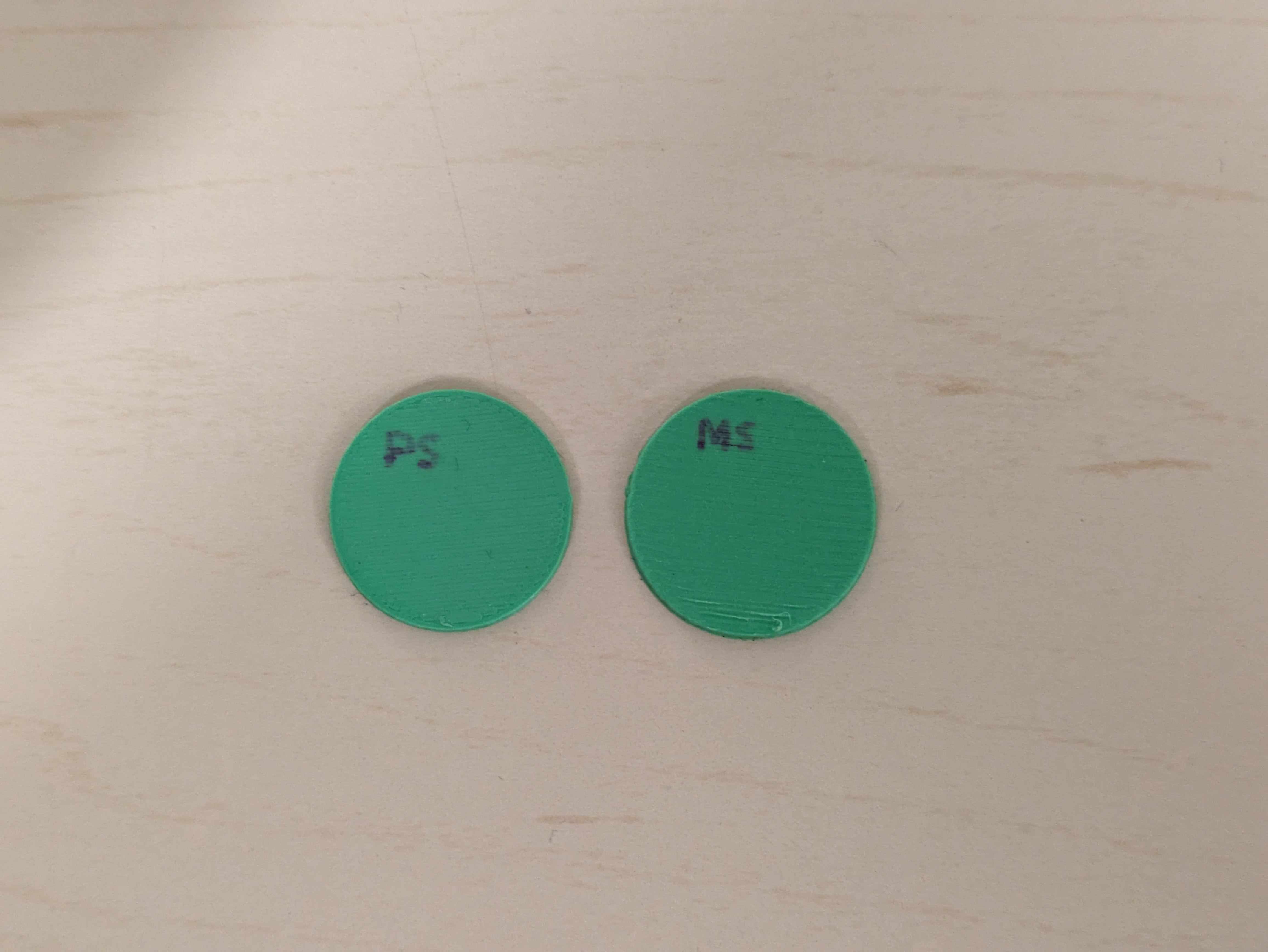
The image below shows two printed objects. The one marked “MS” is my slicer and “PS” is Prusa Slicer. The overall quality of the Prusa Slicer print is better. One key reason is that my slicer draws the infill lines across the outer perimeter. Prusa Slicer ensures that perimeter is printed externally. Another difference is the use of a part cooling fan. Prusa Slicer enables the fan after the first layer and results in better quality. Other things Prusa Slicer is doing are filament retractions and better travel optimization.
Full gcode is here
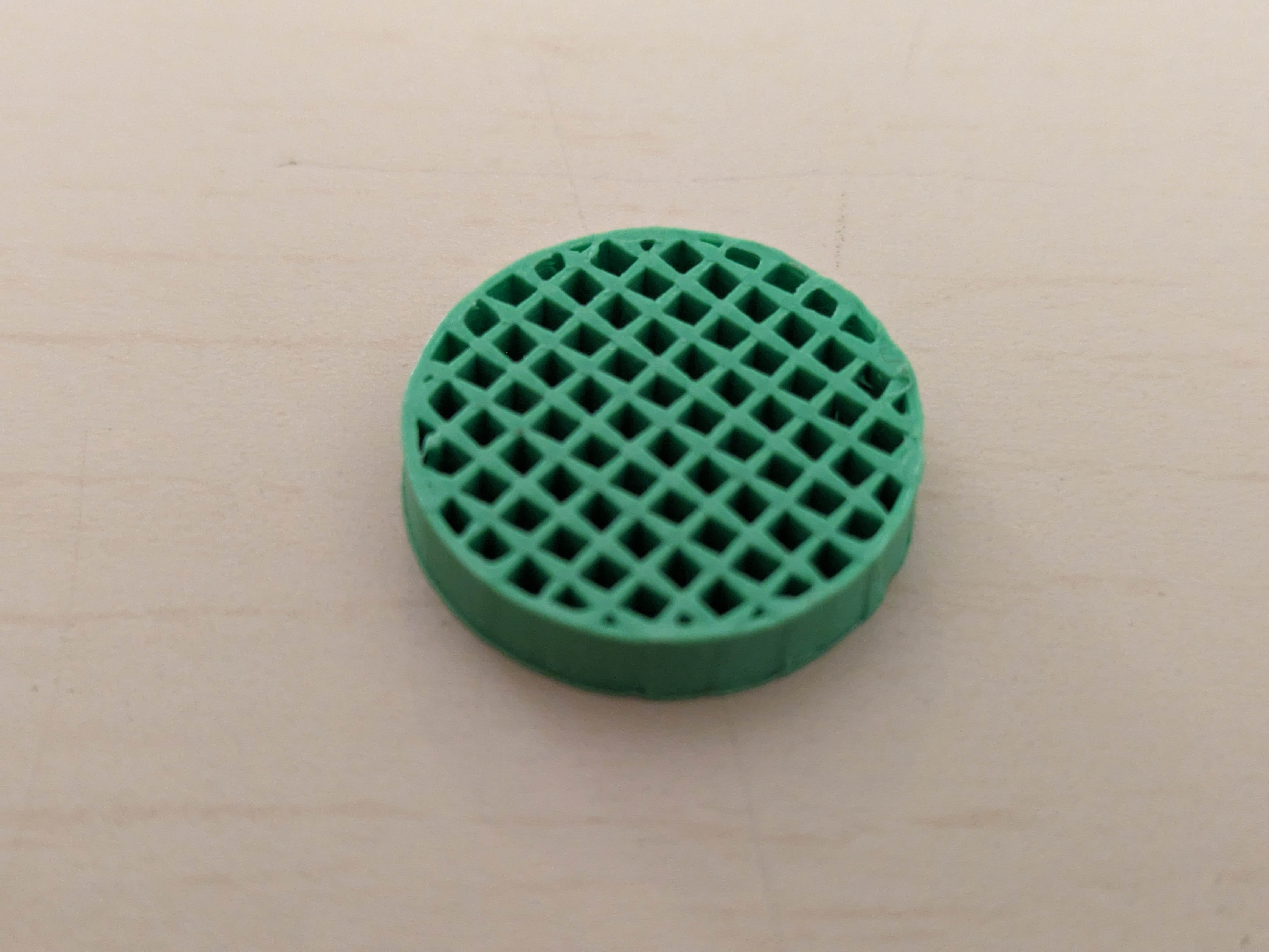
The image below shows a grid infill pattern.
Extra Credit
Infill Density
The infill density can be calculated by first dividing the percentage (out of 100%) by 100.0. Next the bead width is divided by the previous value to determine the line spacing. This is the value that I pass to the generate_lines_infill() function. infill_density = Density / 100.0 line_spacing = bead_wdith / infill_density
The image below shows the result of changing the infill density percentage.

Path Order Optimization
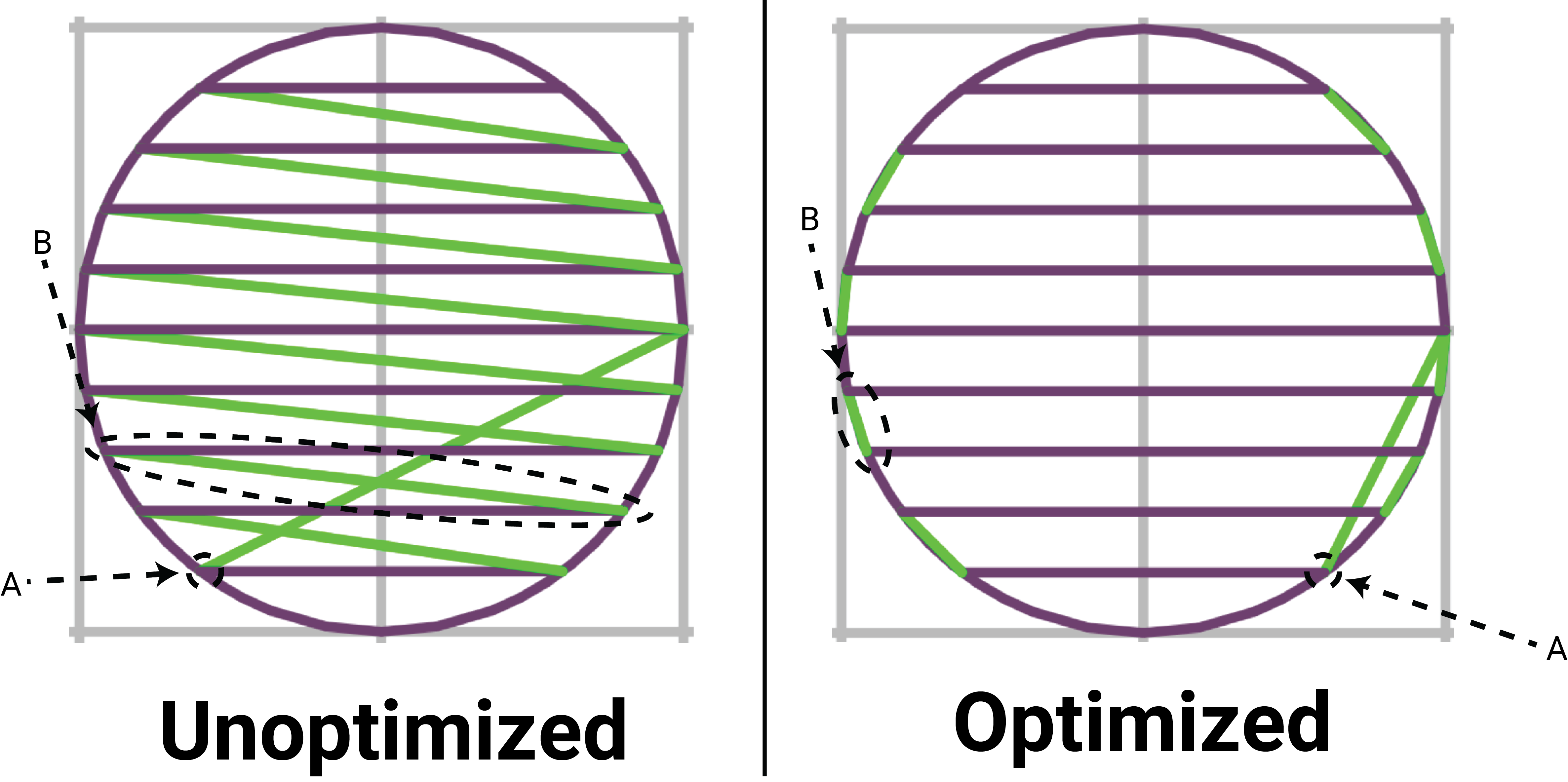
One of the problems with my generated paths is that their relative order is not optimal. The image comparison below details this more. The green lines represent travel moves. From this, we can see that the unoptimized paths have more travel movements. In (B), we can observe that once an infill line is completed, it moves back to the other side to start the next one. Similarly, (A) shows how, when transitioning from the perimeter to the infill, it chooses the wrong end of the first line. The code below presents a simple optimizer to improve this. This code iterates across all the path segments and looks at the next one. If it is more efficient to print the next line in reverse, it flips the start and end coordinates. This process continues for all path segments. The video below shows the correct order while printing.

Infill Patterns: Work in Progresss
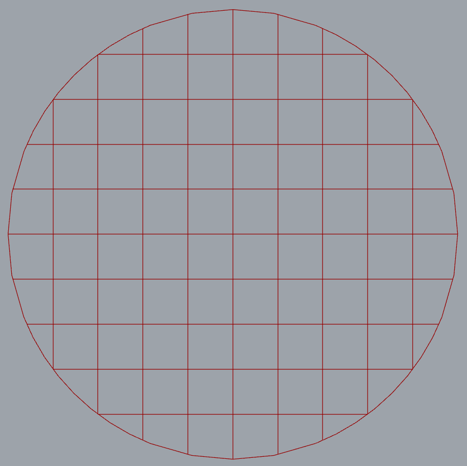
I am still working on infill patterns. I have added a grid infill:
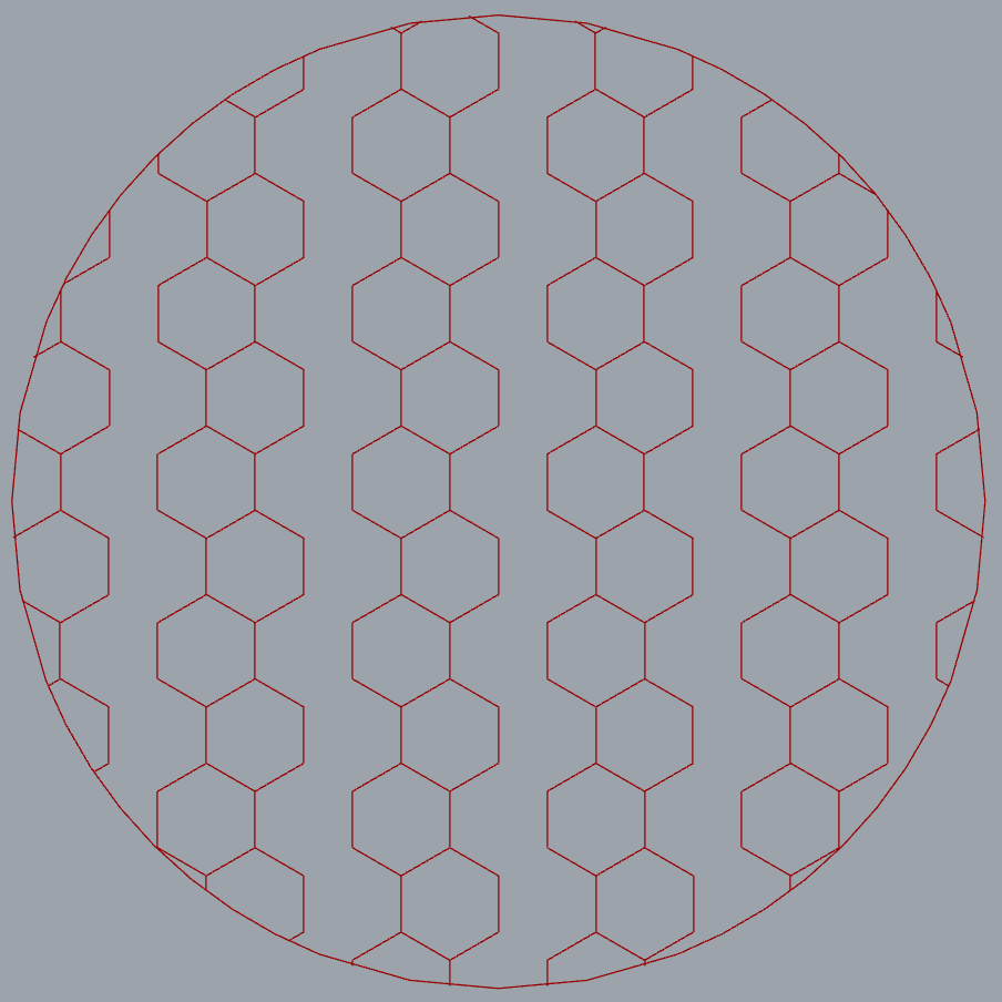
My honeycomb infill it not qite right yet. I am missing some sections.
Vase mdoe:
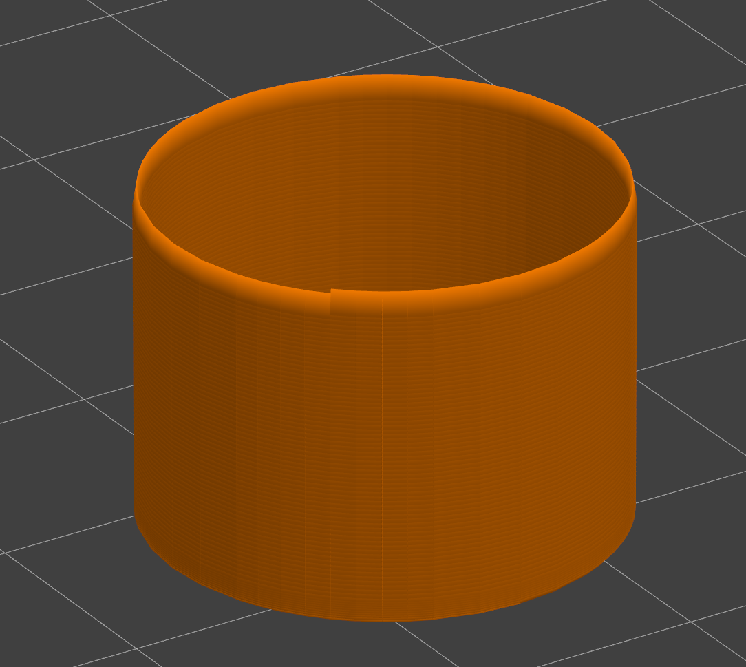
I successfully implemented vase mode in my slicer. To achieve this, I developed an alternative workflow that omits infill generation and path order optimization. This vase mode workflow employs the same code to section an object into perimeters. Each perimeter (Polyline) is then processed through a Python module that applies the vase mode offsets (code provided below).
The script uses two functions. Initially, correct_orientation() is used to ensure all perimeters are wound counter-clockwise, a necessity due to the layer stacking approach of vase mode. The orientation of some perimeters may vary, winding clockwise or counter-clockwise, especially for internal holes of the polygon. Think of the line scanning method and the even/odd rule used to determine if a point lies within the polygon.
Subsequently, the vase_mode() function iteratively adjusts each point in the polyline, incrementing the z-coordinate based on its position along the total perimeter. It begins with the first segment without any extra Z offset, gradually introducing an offset that is one layer height by the last segment. This procedure generates the spiralized effect.
The animation below illustrates the layers being successively stacked, showcasing the spiral effect. Once the Z-offsets have been applied, the path is forwarded to the g-code writer and saved to disk.

